Quick Start
HyperTS is a subtool of DataCanvas AutoML Toolkit(DAT), which is based on the general frameowrk Hypernets. Similar to HyperGBM (another subtool for structured tabular data), HyperTS follows the same rules of both make_experiment API and scikit-learn model API. In general, an experiment is created after the data is ready. Then a trained model can be simply obtained by command run(). To analyze the model, HyperTS also supports the functions like predict(), evaluate() and plot().
The figure below shows the make_experiment workflow of HyperTS:

HyperTS provides the unified API for different tasks, like time series forecasting, classification and regression. An example of how to perform the forecasting task is illustrated as follows.
Data Preparation
This example uses the built-in dataset in HyperTS. Users could load their own datasets by pandas.Dataframe.
from hyperts.datasets import load_network_traffic
from sklearn.model_selection import train_test_split
The data split is based on time sequences to avoid the information leakage. Therefore, the test data is the end part of the whole dataset with setting shuffle=False.
df = load_network_traffic()
train_data, test_data = train_test_split(df, test_size=168, shuffle=False)
df.head()
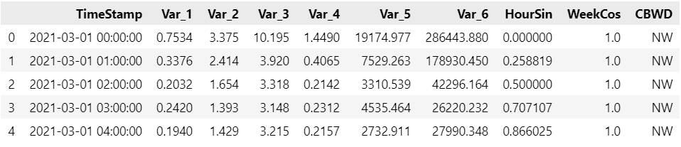
The detail information of this dataset:
The name of the timestampe column is ‘TimeStamp’;
The names of the target columns are ‘Var_1’, ‘Var_2’, ‘Var_3’, ‘Var_4’, ‘Var_5’, ‘Var_6’;
The names of the covariates columns are ‘HourSin’, ‘WeekCos’, ‘CBWD’;
The time frequency is per hour: ‘H’.
Tip
If you have any questions about the data format, please refer to the section Expected Data Format 。
Model Training
An experiment is firsty created by make_experiment with several user-defined parameters. Then the optimal model is simply obtained by using command run(), which integrates the search, training and optimization processes.
from hyperts import make_experiment
experiment = make_experiment(train_data=train_data.copy(),
                            task='forecast',
                            timestamp='TimeStamp',
                            covariables=['HourSin', 'WeekCos', 'CBWD'])
model = experiment.run()
Note
The required parameters for make_experiment are the train_data, task and timestamp, as well as covariables if have. In this case:
The train_data is defined as
train_data=train_data.copy();The task is time series forecasting:
task='forecast';The name of timestamp column is TimeStamp:
timestamp='TimeStamp';The names of the covariates columns are
covariables=['HourSin', 'WeekCos', 'CBWD'];
Tip
For more advanced performance, you could modify other parameters. Please refer to the instructions of Advanced Configurations.
Prediction
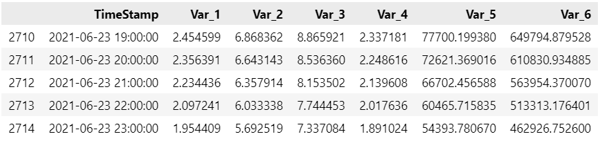
Function split_X_y() is to separate the test data into X (the timestamp and covariates) and y (the target variables). Then perform predict() to obtain the forecast results.
X_test, y_test = model.split_X_y(test_data.copy())
forecast = model.predict(X_test)
forecast.head()
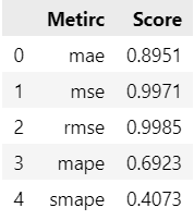
Evaluation
To evaluate the forecast results, use function evaluate() to get the scores of different evaluation criterions. The example below shows the default criterions. Apart from this, users could set the argument metrics to define specific criterions. For instance, metrics=['mae', 'mse', mape_func], where mape_func could be a custom evaluation function or evaluation function from sklearn.
results = model.evaluate(y_true=y_test, y_pred=forecast)
results.head()
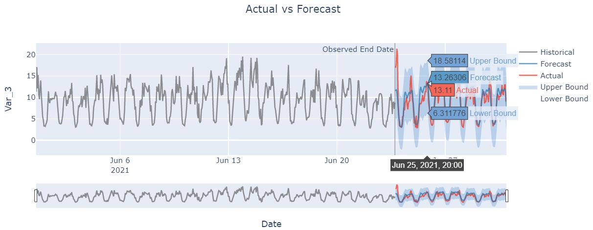
Visualization
Use function plot() to draw the forecast curve and actural result for comparison.
model.plot(forecast=forecast, actual=test_data, interactive=True)
Note
The visualization plot only shows one variable, which is the first target variable by default.
For multivariable forecasting task, user could set the parameter
var_idto plot other target variables. For example,var_id='Var_3'orvar_id=3.The visualization plot supports human interactions: see specific point value and zoom in/out the time scale. The default setting is true,
interactive=true.To plot more historial data, set
history=sub_train_data.When
actual=None(default), it only plots the forecasting curve, without the actural curve.When
show_forecast_interval=True(default), it shows the confidence intervals estimated by Bayesian algorithm.
Tip
The forecasting curve graph is made by plotly library. Users could observe each point value by clicking on the curve.
Save Model
Use function save() to save the trained model.
model.save(model_file="./xxx/xxx/models")
In addition, the second save method can be adopted:
from hyperts.utils.models import save_model

save_model(model=model, model_file="./xxx/xxx/models")
Load Model
Use function load_model() to load the saved model.
from hyperts.utils.models import load_model

pipeline_model = load_model(model_file="./xxx/xxx/models/dl_models")